Choropleth Map: Raw Counts Mostly Redraw the Population Map
The Yardstick Almanac Published No substantive revisions
Short answer
A choropleth map shades each area by one value. In the U.S. county counts we tested, raw totals mostly redrew where people live; dividing by population changed the map.
Station index 7 sections
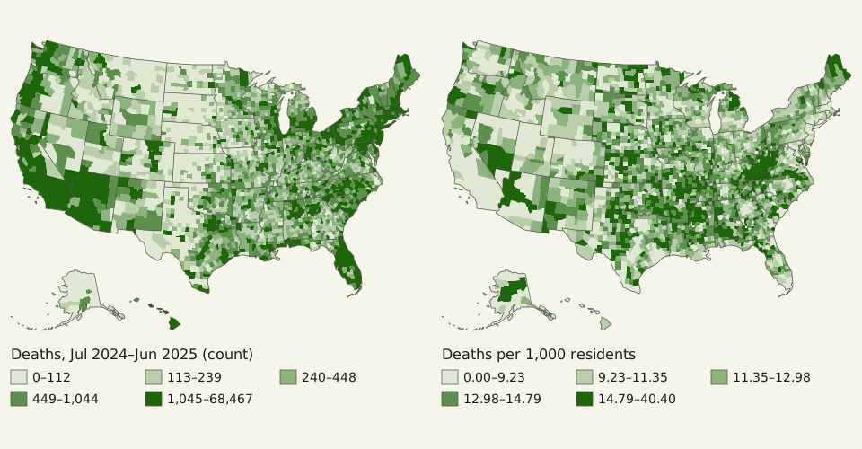
Figure: The Yardstick Almanac, CC BY 4.0
Credit line to copy
"U.S. county deaths as a count and per 1,000 residents" by The Yardstick Almanac, https://theyardstickalmanac.com/maps/choropleth-map/, licensed under CC BY 4.0 (https://creativecommons.org/licenses/by/4.0/).
Data: U.S. Census Bureau, Vintage 2025 county population estimates and components (CO-EST2025-ALLDATA, released March 2026), public domain; U.S. Census Bureau, 2025 cartographic boundary files, counties and states, 1:20,000,000, public domain; drawn 2026-11-01, CC BY 4.0
Rank U.S. counties by yearly deaths, and 8 of the top 10 are also among the 10 most populous. The figures are the Census Bureau's Vintage 2025 county estimates, released in March 2026, which count deaths from July 1, 2024 to June 30, 2025 [measured, source gives no uncertainty]. We shaded all 3,144 counties twice from that one file. This page is about a choice rather than a leftover: what a map divides by, or leaves undivided.
A choropleth map colors each area, such as a county or a state, by one number. If that number is a raw count, big counties win almost by default: deaths, births and business establishments all track county population, with a rank correlation of about 0.98 [estimate, range 0.97–0.99] across the three counts we tested. The denominator the count map leaves out is what we call the unstated per, the “per person” or “per square kilometer” that a number does not say. Divide by residents first and the darkest counties move from big cities to small counties.
What is a choropleth map, and what does it read?
A choropleth map fills each area with a color step, darker for higher values, so the eye reads the whole map as a surface of more and less. The 2007 Census Atlas of the United States gives the rule plainly: “Choropleth maps show derived values such as percentages and medians.” A percentage or a rate has a denominator built in, and a median describes a typical case; a raw count does neither.
The map also weights each county by its land area, not its population. The 737 counties with fewer than 10,000 residents held 1.2 percent of the 2025 population but 32 percent of the land area of all counties. On an equal-area choropleth drawn at one scale, those places fill about a third of the land shown, whatever value they carry.
Florida shows what happens when you skip that step. Its 67 counties are drawn below with the same national class breaks as the maps above. On the count map, Miami-Dade County, with the most deaths in the state, 21,262 [measured, source gives no uncertainty], sits in the darkest class. Its rate was 7.6 per 1,000 residents, below the 9.1 for all counties together.
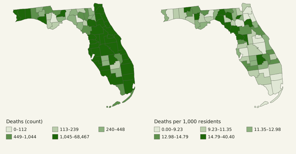
Figure: The Yardstick Almanac, CC BY 4.0
Credit line to copy
"Florida county deaths as a count and per 1,000 residents" by The Yardstick Almanac, https://theyardstickalmanac.com/maps/choropleth-map/, licensed under CC BY 4.0 (https://creativecommons.org/licenses/by/4.0/).
Data: U.S. Census Bureau, Vintage 2025 county population estimates and components (CO-EST2025-ALLDATA, released March 2026), public domain; U.S. Census Bureau, 2025 cartographic boundary files, counties and states, 1:20,000,000, public domain; drawn 2026-11-01, CC BY 4.0
On the rate map the dark counties are different ones. Citrus County had the highest rate in Florida, 18.0 per 1,000, and Sumter County was fourth at 17.0. These are crude rates: deaths per resident, with no adjustment for age. The federal mortality atlas discussed below maps age-adjusted rates instead, which answers yet another question.
Our death rate uses the Census Bureau's own denominator, and that denominator is itself a choice. The file layout divides each year's deaths by “the average of the July 1 beginning and ending resident total populations,” then multiplies by 1,000. Our rate matched the published one in every county.
Why do raw-count maps look like population maps?
Most things counted per county happen to people, and people are spread very unevenly across the 3,144 counties. Plot each county's count against its population on log axes and the dots form a narrow band.
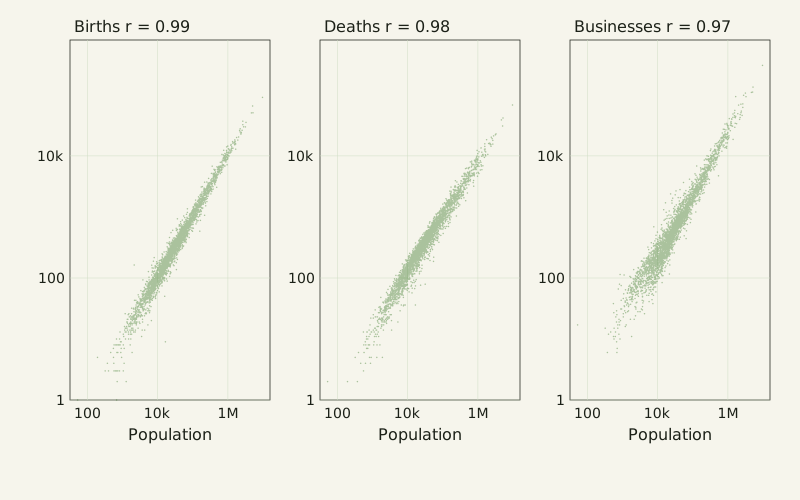
Figure: The Yardstick Almanac, CC BY 4.0
Credit line to copy
"Births, deaths and business establishments against county population" by The Yardstick Almanac, https://theyardstickalmanac.com/maps/choropleth-map/, licensed under CC BY 4.0 (https://creativecommons.org/licenses/by/4.0/).
Data: U.S. Census Bureau, Vintage 2025 county population estimates and components (CO-EST2025-ALLDATA, released March 2026), public domain; U.S. Census Bureau, County Business Patterns 2023, county file, public domain; drawn 2026-11-01, CC BY 4.0
| County count | Data year | Rank correlation with population | Shared with the 10 most populous | Shared with the 100 most populous |
|---|---|---|---|---|
| Births | Jul 2024–Jun 2025 | 0.987 | 9 of 10 | 94 of 100 |
| Deaths | Jul 2024–Jun 2025 | 0.982 | 8 of 10 | 85 of 100 |
| Business establishments | 2023 | 0.969 | 8 of 10 | 91 of 100 |
| Net domestic migration | Jul 2024–Jun 2025 | 0.241 | 0 of 10 | 13 of 100 |
The last row is where the rule stops. Net domestic migration is a flow that can be negative, and big counties often lose people to the rest of the country. So the claim is “mostly,” not “in every case”: in our data, counts of things that happen to residents or businesses tracked population closely.
On the quintile maps, all 100 of the most populous counties fall in the darkest class of the death-count map. On the map of deaths per 1,000 residents, none of them do. Across all counties, the rank correlation between the death rate and population is −0.46: the rate runs the other way.
Per resident or per square kilometer?
Each denominator answers a different question. Per resident asks how common deaths were among the people who live there. Per square kilometer of land asks how densely they were packed onto the ground. The second one mostly brings the population map back.
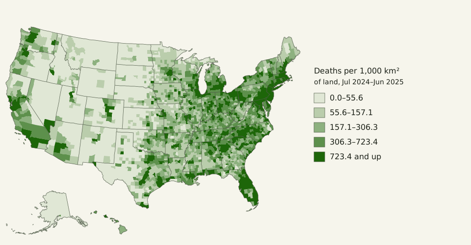
Figure: The Yardstick Almanac, CC BY 4.0
Credit line to copy
"U.S. county deaths per 1,000 km² of land" by The Yardstick Almanac, https://theyardstickalmanac.com/maps/choropleth-map/, licensed under CC BY 4.0 (https://creativecommons.org/licenses/by/4.0/).
Data: U.S. Census Bureau, Vintage 2025 county population estimates and components (CO-EST2025-ALLDATA, released March 2026), public domain; U.S. Census Bureau, 2025 cartographic boundary files, counties and states, 1:20,000,000, public domain; drawn 2026-11-01, CC BY 4.0
Deaths per 1,000 km2 and residents per km2 have a rank correlation of 0.99 across counties, and 9 of the top 10 counties are the same on both lists. That map is a density map wearing a mortality label. It suits questions about the land itself and is the wrong tool for asking where death was unusually common.
The question “per what?” shows up well beyond maps. Shares can switch with the denominator: the 1884 meridian debate quoted Greenwich's lead in ships and in tonnage, which gave two different percentages, as told in the prime meridian vote. Even a birthday count depends on it, as in how many people are born on February 29, where the odds differ per calendar day and per birth.
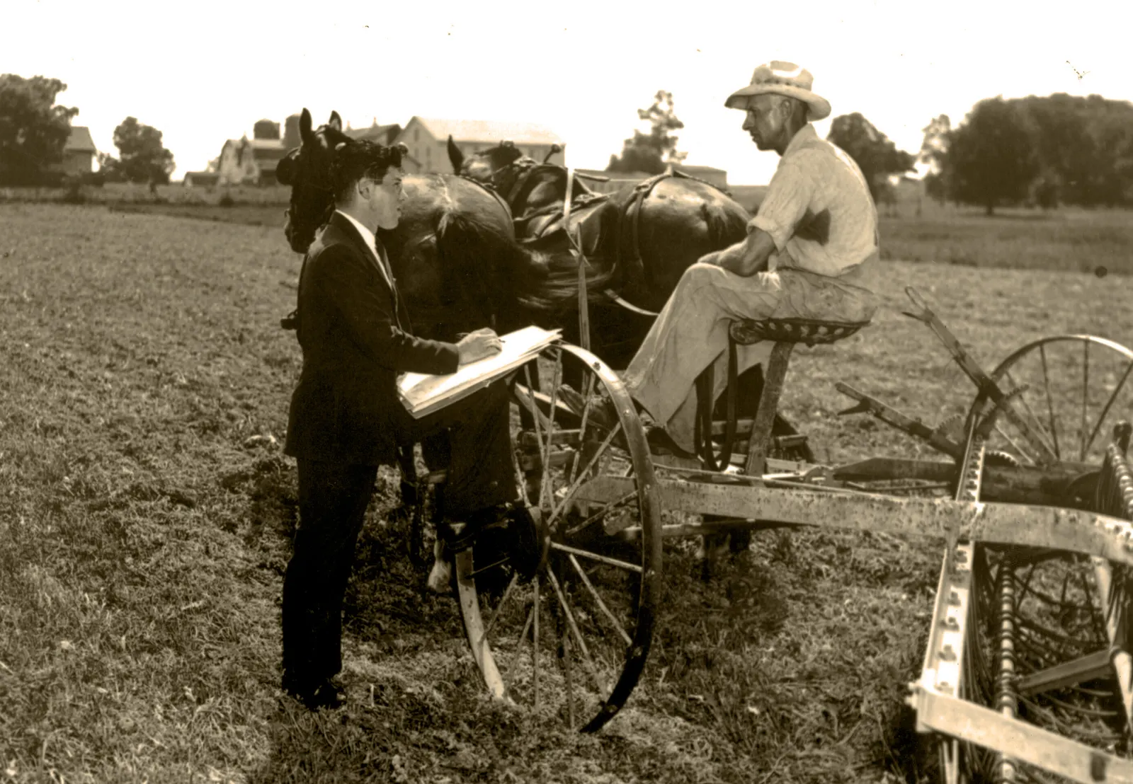
"1940 Census Enumeration" by U.S. Census Bureau, public domain
Full credit
"1940 Census Enumeration" by U.S. Census Bureau — https://commons.wikimedia.org/wiki/File:1940_Census_Enumeration_(5020520332).jpg — Public domain (work of the U.S. federal government, 17 U.S.C. §105: the Commons file page tags it as the work of a United States Census Bureau employee made as part of official duties; also released by the U.S. Census Bureau on Flickr under CC BY 2.0, which is the basis used outside the United States)
How do class breaks change the story?
The same rates can be cut into five colors in more than one way. Quintile classes put about a fifth of the counties in each color, 628 or 629 each here. Equal-interval classes split the range from the lowest rate to the highest into five equal steps.
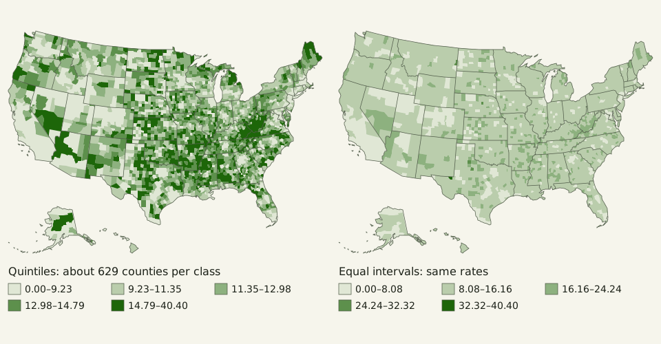
Figure: The Yardstick Almanac, CC BY 4.0
Credit line to copy
"County death rates in quintile and equal-interval classes" by The Yardstick Almanac, https://theyardstickalmanac.com/maps/choropleth-map/, licensed under CC BY 4.0 (https://creativecommons.org/licenses/by/4.0/).
Data: U.S. Census Bureau, Vintage 2025 county population estimates and components (CO-EST2025-ALLDATA, released March 2026), public domain; U.S. Census Bureau, 2025 cartographic boundary files, counties and states, 1:20,000,000, public domain; drawn 2026-11-01, CC BY 4.0
The rates run from 0.0 to 40.4 per 1,000, and the top of that range comes from one county, Loving County, Texas, with 52 residents and 2 deaths [measured, source gives no uncertainty]. Equal intervals let that single value set the scale: 2,463 counties land in the second class, 4 in the fourth and only Loving in the fifth, so the map turns mostly into one color.
Quintiles do the opposite. They spend the colors evenly, so they show contrast by design, even where the real differences are small. The breaks depend only on rank order, and a reader cannot tell from the colors alone whether neighboring classes differ by 0.1 or by 10. Printing each class range in the legend, and in the data file, lets the reader see the steps the colors hide.
The Census Atlas took a third route: its class breaks “were chosen using a combination of national rates and rounded breaks shared among maps for each topic.” Fixed, shared breaks let readers compare one map with the next, which neither quintiles nor equal intervals can promise. Color is not the only cue that can mislead, either. Pie charts raise the same question of which cue the eye judges, as covered in how readers judge pie slices.
What did the federal atlases find?
Two U.S. government atlases describe how they chose to map counts and rates, and both are public documents whose relevant chapters we read in full.
The Atlas of United States Mortality, published in 1996 by the National Center for Health Statistics, tested map styles before choosing one. Its methods chapter reports that experiments with shaded areas, symbols, dot density and contour lines “showed the clear advantage of classed (categorized rate) choropleth maps over competing map styles.” Those experiments are summarized in the atlas; we did not read the underlying studies. The same chapter says single-hue steps of darkness helped readers spot “clusters or broad patterns.”
The same atlas also gives the strongest case against mapping county rates naively. For many causes of death, it says, the data “are too sparse to provide stable 5-year rates at the county level.” Its authors mapped 805 health service areas instead of 3,141 counties, and our own data shows why that compromise made sense.
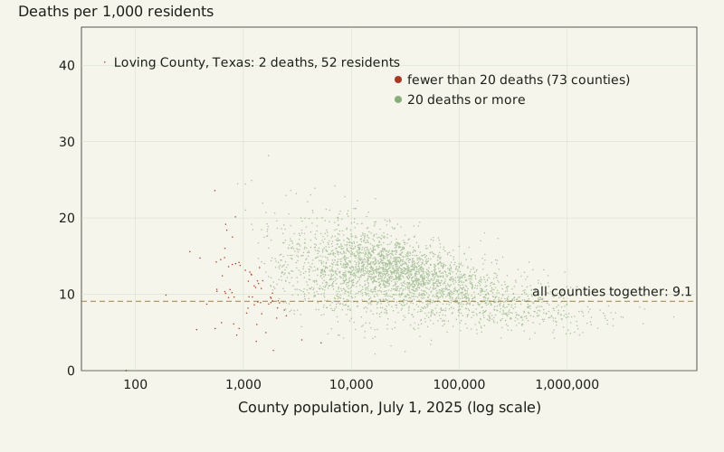
Figure: The Yardstick Almanac, CC BY 4.0
Credit line to copy
"County death rate against county population" by The Yardstick Almanac, https://theyardstickalmanac.com/maps/choropleth-map/, licensed under CC BY 4.0 (https://creativecommons.org/licenses/by/4.0/).
Data: U.S. Census Bureau, Vintage 2025 county population estimates and components (CO-EST2025-ALLDATA, released March 2026), public domain; drawn 2026-11-01, CC BY 4.0
The 73 counties with fewer than 20 deaths had rates from 0.0 to 40.4 per 1,000. Counties with 20 deaths or more stayed between 2.2 and 28.2. A rate built on two deaths rises by half with one more death, yet a choropleth gives that tiny county the same visual weight as any other county of its size.
The Census Atlas splits the job between two map types. Its key to map types says choropleth maps are for derived values, while “graduated symbol maps show numbers of people or other quantities,” with larger symbols for higher values.
Choropleth map questions
How do I check a choropleth before trusting it?
- Read the legend title and ask “per what?” If the value is a plain total, expect the map to follow population.
- Find the class ranges. Check whether the classes hold equal numbers of areas, equal steps of value, or breaks chosen by hand.
- Look for the smallest areas with the darkest colors. A rate built on a handful of cases can land in the top class by chance.
- Check the date of the data and the date of the boundaries, since counties are sometimes redrawn.
- Look at a table or the data file behind the map before quoting any single area.
Is a choropleth the same as a heat map?
Not in the Census Atlas's terms. A choropleth fills fixed areas, such as counties, with one color each. The atlas describes a different type, the isoplethic map, which “gives an impression of continuous population distribution” by drawing lines that connect equal values. If a map blends color smoothly across county lines, it is closer to that second type than to a choropleth.
Should a choropleth use rates or counts?
Use a derived value: a rate, a share or a median. The atlas's wording names percentages and medians, and a rate per 1,000 residents is the same kind of number, while plain counts go on its graduated symbol maps. If you must shade counts, say so in the legend and expect the result to follow population.
What projection do these maps use?
Every map here uses an Albers equal-area conic projection, which keeps areas in proportion so large counties are not inflated. The 48 conterminous states and Washington, D.C., use standard parallels of 29.5° N and 45.5° N, with the origin at 23° N, 96° W. Alaska is drawn in its own Albers projection at 0.35 of the main scale, and Hawaii in a third at the same scale. Boundaries come from the Census Bureau's 2025 county file, made for maps at about 1:20,000,000.
When is a count map the right map?
When the question really is “how many,” keep the count and change the symbol. A proportional symbol map puts one circle in each county, with the circle's area set by the count, so a big circle in a small county reads correctly as many deaths in a small place.
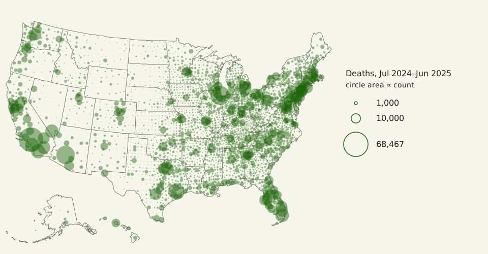
Figure: The Yardstick Almanac, CC BY 4.0
Credit line to copy
"U.S. county deaths as proportional circles" by The Yardstick Almanac, https://theyardstickalmanac.com/maps/choropleth-map/, licensed under CC BY 4.0 (https://creativecommons.org/licenses/by/4.0/).
Data: U.S. Census Bureau, Vintage 2025 county population estimates and components (CO-EST2025-ALLDATA, released March 2026), public domain; U.S. Census Bureau, 2025 cartographic boundary files, counties and states, 1:20,000,000, public domain; drawn 2026-11-01, CC BY 4.0
| Map | What it answers | Main risk |
|---|---|---|
| Choropleth of a raw count | Which large areas hold the most | Mostly redraws population; big counties dominate |
| Choropleth per 1,000 residents | Where something is common among residents | Small counties give unstable rates |
| Choropleth per km² of land | Where it is packed densely on the ground | Mostly redraws population density |
| Proportional symbols | How many, and where | Circles overlap in crowded regions |
Position: a choropleth of raw counts is usually a population map in disguise, and it should be redrawn as a rate or as symbols. The limit of that position is the small-number problem: where counts are tiny, a rate map needs wider areas, several years pooled, or a note on which counties rest on few cases. We take apart charts and maps, not the people who make them.
The table below lists the ten counties with the most deaths and the ten with the highest rates. None of the ten highest-rate counties is among the ten most populous, and all ten have fewer than 7,100 residents.
| Rank | Most deaths (count) | Deaths | Highest deaths per 1,000 | Rate | Residents |
|---|---|---|---|---|---|
| 1 | Los Angeles County, CA | 68,467 | Loving County, TX | 40.4 | 52 |
| 2 | Cook County, IL | 41,853 | Garfield County, NE | 28.2 | 1,710 |
| 3 | Maricopa County, AZ | 38,883 | Stonewall County, TX | 24.9 | 1,186 |
| 4 | Harris County, TX | 30,892 | Wibaux County, MT | 24.5 | 885 |
| 5 | San Diego County, CA | 22,951 | Motley County, TX | 24.4 | 1,043 |
| 6 | Orange County, CA | 22,178 | Kingman County, KS | 24.2 | 7,029 |
| 7 | Miami-Dade County, FL | 21,262 | Hot Springs County, WY | 23.9 | 4,600 |
| 8 | Clark County, NV | 20,315 | Real County, TX | 23.6 | 2,745 |
| 9 | Riverside County, CA | 19,249 | McMullen County, TX | 23.6 | 544 |
| 10 | Wayne County, MI | 18,472 | Sharkey County, MS | 23.2 | 3,097 |
Sources
- U.S. Census Bureau, Population Division, “Annual Resident Population Estimates, Estimated Components of Resident Population Change, and Rates of the Components of Resident Population Change for States and Counties: April 1, 2020 to July 1, 2025” (CO-EST2025-ALLDATA), Vintage 2025, released March 2026. https://www2.census.gov/programs-surveys/popest/datasets/2020-2025/counties/totals/co-est2025-alldata.csv Read: full dataset
- U.S. Census Bureau, “CO-EST2025-ALLDATA: Annual Resident Population Estimates, Estimated Components of Resident Population Change, and Rates of the Components of Resident Population Change for States and Counties: April 1, 2020 to July 1, 2025,” file layout. https://www2.census.gov/programs-surveys/popest/technical-documentation/file-layouts/2020-2025/CO-EST2025-ALLDATA.pdf Read: full text
- U.S. Census Bureau, County Business Patterns 2023, county file (cbp23co), with the county data dictionary and the NAICS code list (“------”: Total for all sectors). https://www2.census.gov/programs-surveys/cbp/datasets/2023/cbp23co.zip Read: full dataset
- U.S. Census Bureau, 2025 Cartographic Boundary Files, counties and states, 1:20,000,000 (cb_2025_us_county_20m, cb_2025_us_state_20m). https://www2.census.gov/geo/tiger/GENZ2025/shp/ Read: full dataset
- U.S. Census Bureau, Census Atlas of the United States, Series CENSR-29 (Washington, D.C., 2007), chapter 1, “Introduction.” https://www.census.gov/library/publications/2007/dec/censr-29.html Read: full chapter (chapter 1)
- Linda Williams Pickle, Michael Mungiole, Gretchen K. Jones and Andrew A. White, Atlas of United States Mortality (Hyattsville, MD: National Center for Health Statistics, 1996), DHHS Publication No. (PHS) 97-1015. https://www.cdc.gov/nchs/data/misc/atlasmet.pdf Read: methods chapter, full text
Data files (counts and rates for every county computed from the Census Bureau files with Python and pandas, cross-checked by a second independent computation; maps drawn in an Albers equal-area projection; CC BY 4.0):
- Every county: population, deaths, births, establishments, rates, land area and map classes (CSV) (CSV, source and license notes) Data: U.S. Census Bureau, Vintage 2025 county population estimates and components (CO-EST2025-ALLDATA, released March 2026), public domain; U.S. Census Bureau, County Business Patterns 2023, county file, public domain; U.S. Census Bureau, 2025 cartographic boundary files, counties and states, 1:20,000,000, public domain; computed 2026-11-01, CC BY 4.0
- How four county counts follow population (CSV) (CSV, source and license notes) Data: U.S. Census Bureau, Vintage 2025 county population estimates and components (CO-EST2025-ALLDATA, released March 2026), public domain; U.S. Census Bureau, County Business Patterns 2023, county file, public domain; computed 2026-11-01, CC BY 4.0
- Class breaks for the quintile and equal-interval maps (CSV) (CSV, source and license notes) Data: U.S. Census Bureau, Vintage 2025 county population estimates and components (CO-EST2025-ALLDATA, released March 2026), public domain; computed 2026-11-01, CC BY 4.0
- What the two federal atlases say, with how much of each was read (CSV) (CSV, source and license notes) Data: U.S. Census Bureau, Census Atlas of the United States (2007), chapter 1, public domain; National Center for Health Statistics, Atlas of United States Mortality (1996), public domain; computed 2026-11-01, CC BY 4.0
Cite this page
The Yardstick Almanac. "Choropleth Map: Raw Counts Mostly Redraw the Population Map." Published November 1, 2026. https://theyardstickalmanac.com/maps/choropleth-map/. Accessed [the date you read it].
More in Maps Explained
Maps Explained
Prime Meridian: The 1884 Vote Named a Telescope, Not a Mark
Image credit
"The Royal Observatory, Greenwich Hill, top, and the view of Greenwich and London seen from the hill, below" by Wellcome Collection — https://commons.wikimedia.org/wiki/File:The_Royal_Observatory,_Greenwich_Hill,_top,_and_the_view_of_Wellcome_V0013355.jpg — CC BY 4.0 (https://creativecommons.org/licenses/by/4.0/)

Maps Explained
WGS 84: The Same Coordinates Can Land Meters Apart
Image credit
"Global Positioning System satellite" by Scott Ehardt — https://commons.wikimedia.org/wiki/File:Global_Positioning_System_satellite.jpg — Public domain (Author dedication, not term expiry: the photographer, Scott Ehardt, released this own work (uploaded 2 June 2005) into the public domain worldwide on the Commons file page, so it holds in the United States and in the EU alike; where a dedication is not legally possible, his fallback grant lets anyone use the work for any purpose without conditions. The photographed object is an unlaunched GPS Block II-A satellite, a utilitarian spacecraft on museum display, not a separate artwork.)
How this page is checked: Where the numbers come from explains the value tags, the source order and how every figure is recomputed.
Corrections: every substantive change is logged in What we got wrong.
Spotted an error? Email contact@theyardstickalmanac.com with the sentence and your source, or read Write in first.